Text Modeling and Analysis using Quanteda
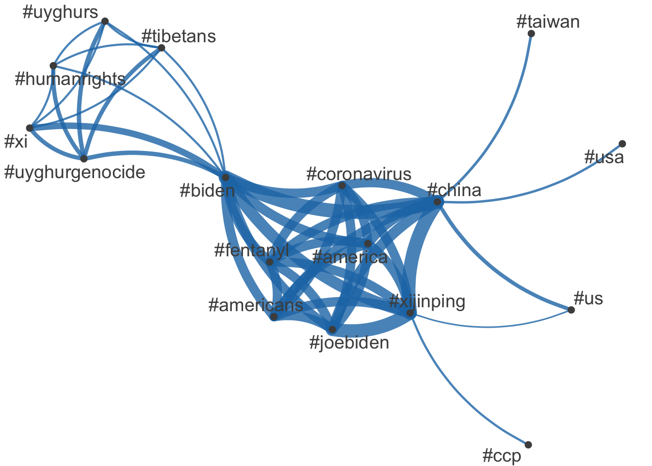
This document demonstrates how to perform text modeling and analysis using the quanteda package. We use data from various sources, including US presidential inaugural addresses and tweets about the Biden-Xi summit in November 2021.
Installation of Required Packages
# Set the CRAN mirror options (repos = c (CRAN = "https://cran.rstudio.com/" ))install.packages (c ("quanteda" , "quanteda.textmodels" , "quanteda.textplots" , "quanteda.textstats" , "readr" , "ggplot2" ))
The downloaded binary packages are in
    /var/folders/m3/k788kw6103zdvc0bwpc1lzd00000gn/T//RtmpxxEMOr/downloaded_packages
library (quanteda)library (quanteda.textmodels)library (quanteda.textplots)library (quanteda.textstats)library (readr)library (ggplot2)
Latent Semantic Analysis (LSA)
Latent Semantic Analysis (LSA) is a technique used to reduce the dimensionality of text data. Here, we apply LSA to the tweet data.
<- textmodel_lsa (sumtwtdfm)summary (sum_lsa)
                Length    Class     Mode
sk                     10 -none-    numeric
docs               145200 -none-    numeric
features           159930 -none-    numeric
matrix_low_rank 232218360 -none-    numeric
data            232218360 dgCMatrix S4
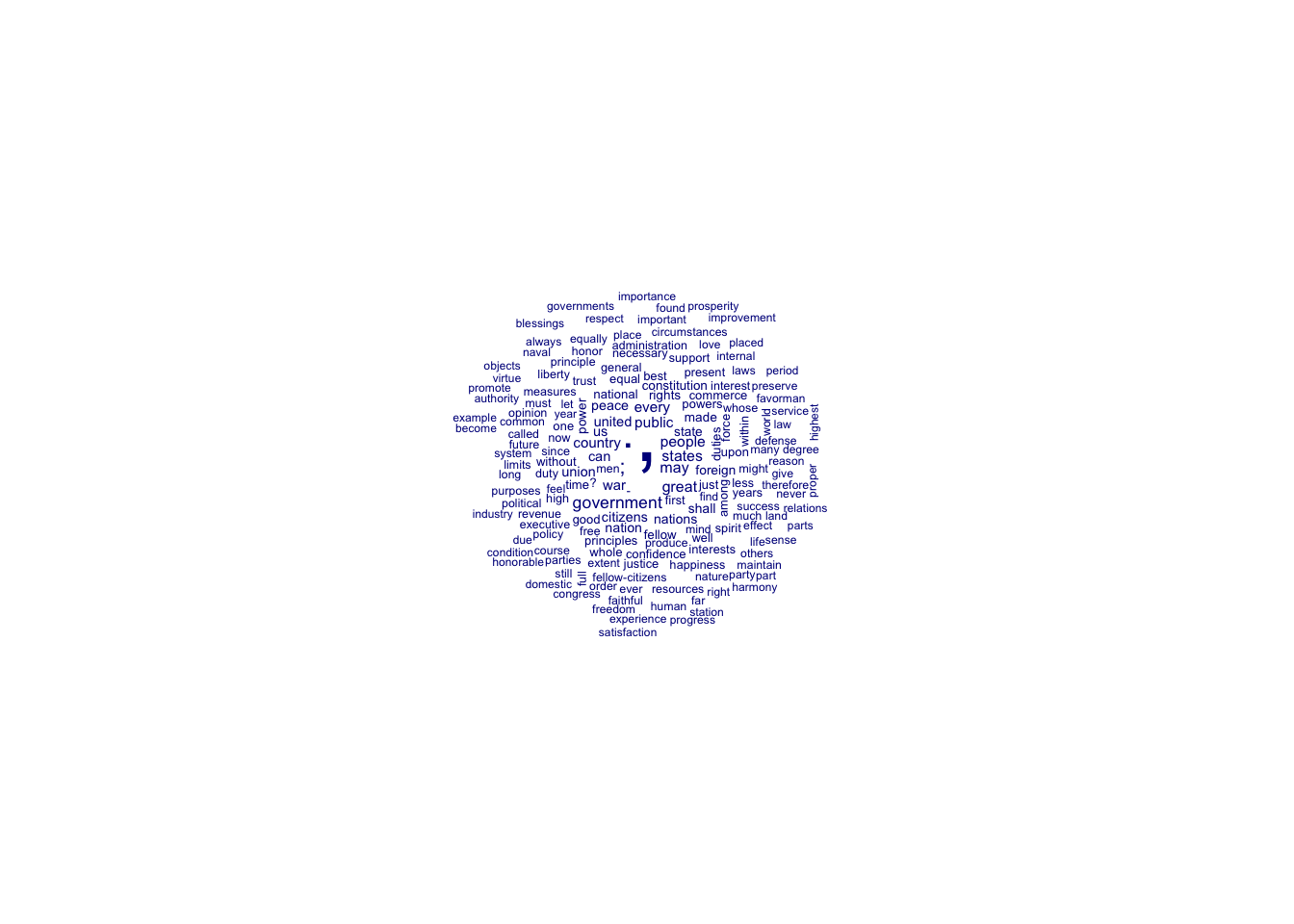
Wordcloud from US Presidential Inaugural Addresses
The following code generates a word cloud based on US presidential inaugural addresses from 1789 to 1826.
<- corpus_subset (data_corpus_inaugural, Year <= 1826 ) %>% tokens () %>% dfm () %>% dfm_remove (stopwords ('english' )) %>% dfm_remove (pattern = "[[:punct:]]" ) %>% dfm_trim (min_termfreq = 10 , verbose = FALSE )set.seed (100 )textplot_wordcloud (dfm_inaug)
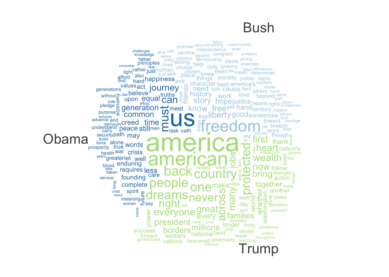
Comparison Wordcloud for Recent Presidents
We can compare the word usage of different presidents in their inaugural speeches using a word cloud.
corpus_subset (data_corpus_inaugural, %in% c ("Trump" , "Obama" , "Bush" )) %>% tokens (remove_punct = TRUE ) %>% tokens_remove (stopwords ("english" )) %>% dfm () %>% dfm_group (groups = President) %>% dfm_trim (min_termfreq = 5 , verbose = FALSE ) %>% textplot_wordcloud (comparison = TRUE )
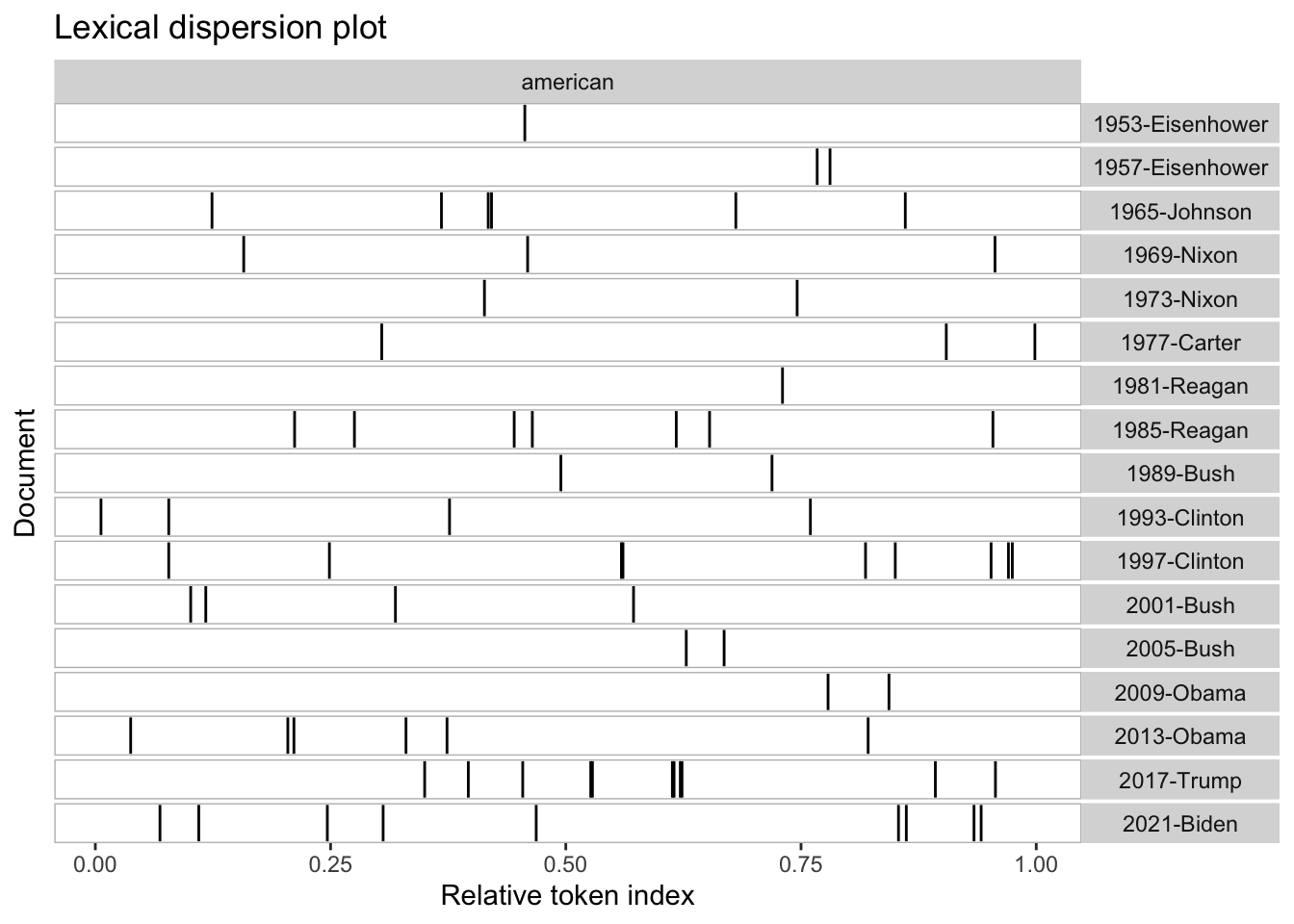
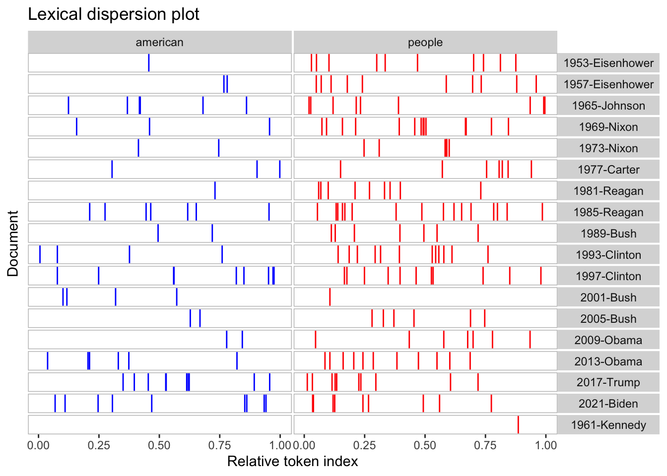
Keyword in Context (KWIC) Analysis
We can use Keyword in Context (KWIC) analysis to see how specific terms, such as “american”, “people”, and “communist” are used in speeches after 1949.
<- corpus_subset (data_corpus_inaugural, Year > 1949 )<- tokens (data_corpus_inaugural_subset)# Perform KWIC analysis for the word "american" kwic (kwic_tokens, pattern = "american" ) %>% textplot_xray ()# Plot KWIC for multiple words <- textplot_xray (kwic (kwic_tokens, pattern = "american" ),kwic (kwic_tokens, pattern = "people" ),kwic (kwic_tokens, pattern = "communist" )+ aes (color = keyword) + scale_color_manual (values = c ("blue" , "red" , "green" )) + theme (legend.position = "none" )
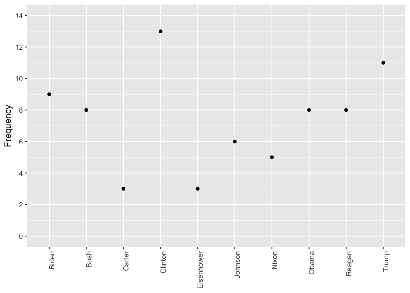
Frequency of Terms
Here, we analyze the frequency of the term “american” across different presidents’ speeches.
<- textstat_frequency (dfm (tokens (data_corpus_inaugural_subset)), groups = data_corpus_inaugural_subset$ President)<- subset (freq_grouped, freq_grouped$ feature %in% "american" ) ggplot (freq_american, aes (x = group, y = frequency)) + geom_point () + scale_y_continuous (limits = c (0 , 14 ), breaks = c (seq (0 , 14 , 2 ))) + xlab (NULL ) + ylab ("Frequency" ) + theme (axis.text.x = element_text (angle = 90 , hjust = 1 ))
Warning: Removed 1 row containing missing values or values outside the scale range
(`geom_point()`).
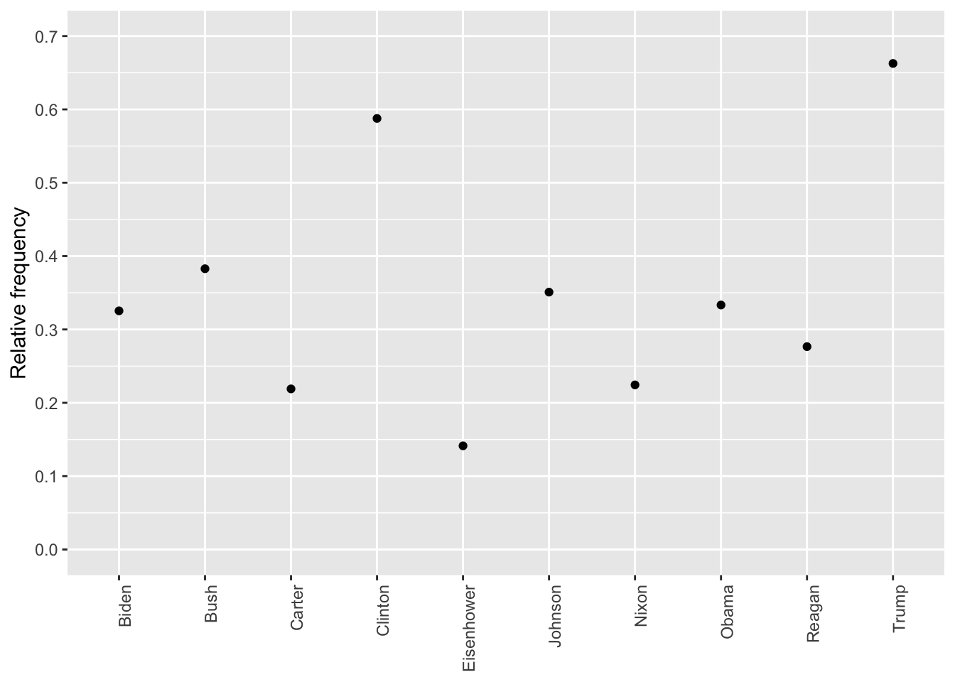
Relative Frequency of Terms
The following code calculates the relative frequency of the term “american” across different presidents.
<- dfm_weight (dfm (tokens (data_corpus_inaugural_subset)), scheme = "prop" ) * 100 <- textstat_frequency (dfm_rel_freq, groups = dfm_rel_freq$ President)<- subset (rel_freq, feature %in% "american" ) ggplot (rel_freq_american, aes (x = group, y = frequency)) + geom_point () + scale_y_continuous (limits = c (0 , 0.7 ), breaks = c (seq (0 , 0.7 , 0.1 ))) + xlab (NULL ) + ylab ("Relative frequency" ) + theme (axis.text.x = element_text (angle = 90 , hjust = 1 ))
Warning: Removed 1 row containing missing values or values outside the scale range
(`geom_point()`).
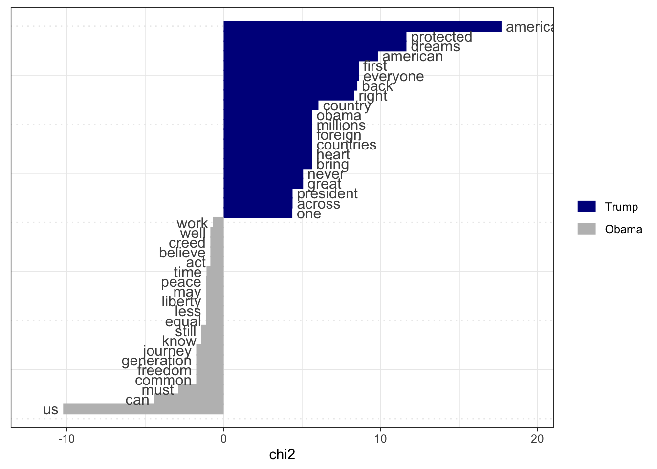
Keyness Analysis for Obama and Trump Speeches
We compare the key terms in the inaugural speeches of Obama and Trump using keyness analysis.
<- corpus_subset (data_corpus_inaugural, %in% c ("Obama" , "Trump" ))<- tokens (pres_corpus, remove_punct = TRUE ) %>% tokens_remove (stopwords ("english" )) %>% tokens_group (groups = President) %>% dfm ()<- textstat_keyness (pres_dfm, target = "Trump" )# Plot estimated word keyness textplot_keyness (result_keyness)
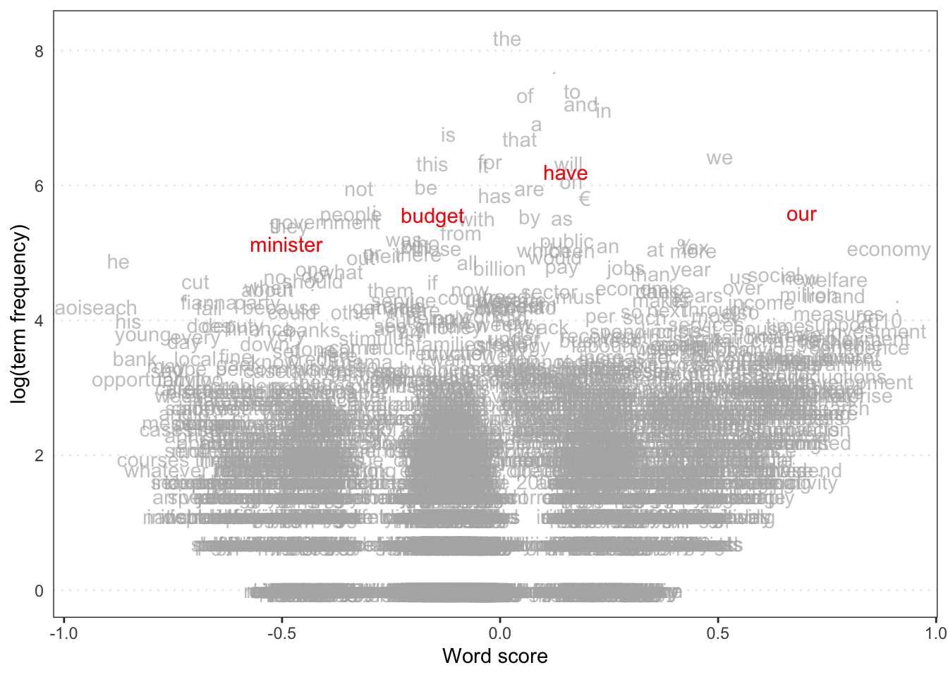
Wordscores Model
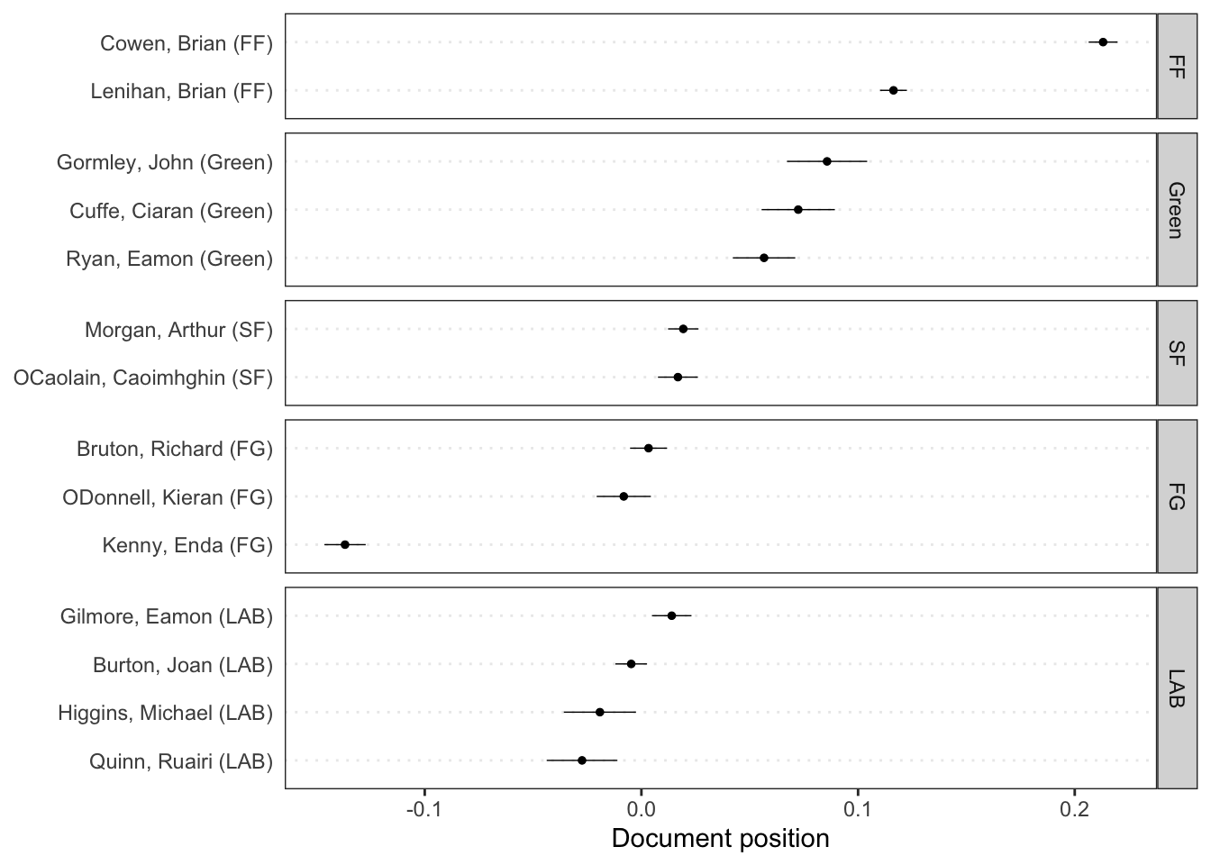
We can estimate word positions and predictions using a Wordscores model.
data (data_corpus_irishbudget2010, package = "quanteda.textmodels" )<- dfm (tokens (data_corpus_irishbudget2010))<- c (rep (NA , 4 ), 1 , - 1 , rep (NA , 8 ))<- textmodel_wordscores (ie_dfm, y = refscores, smooth = 1 )# Plot estimated word positions textplot_scale1d (ws, highlighted = c ("minister" , "have" , "our" , "budget" ), highlighted_color = "red" )# Get predictions and plot document positions <- predict (ws, se.fit = TRUE )textplot_scale1d (pred, margin = "documents" , groups = docvars (data_corpus_irishbudget2010, "party" ))