Lab05 Linear Regression Lab

Author

Jim

1 Introduction

This document demonstrates various linear regression techniques using the Boston and Carseats datasets. We will explore simple linear regression, multiple linear regression, interaction terms, and nonlinear terms. The tutorial will also cover plotting regression results and interpreting qualitative predictors.

2 Setup

First, we need to install and load the required packages and datasets.

# Setup CRAN Mirror
options(repos = c(CRAN = "https://cran.rstudio.com/"))

install.packages(c("easypackages", "MASS", "ISLR", "arm"))

The downloaded binary packages are in
    /var/folders/m3/k788kw6103zdvc0bwpc1lzd00000gn/T//RtmpO1X8f3/downloaded_packages
library(easypackages)
libraries("arm", "MASS", "ISLR")

3 Load the Dataset

We start by attaching the Boston dataset, which contains housing data used to predict median home values (medv).

attach(Boston)

4 Simple Linear Regression

We will fit a simple linear regression model to predict medv using lstat (the percentage of lower-income population).

plot(medv ~ lstat, Boston, pch = 20, cex = .8, col = "steelblue")
fit1 = lm(medv ~ lstat, data = Boston)
summary(fit1)

Call:
lm(formula = medv ~ lstat, data = Boston)

Residuals:
    Min      1Q  Median      3Q     Max 
-15.168  -3.990  -1.318   2.034  24.500 

Coefficients:
            Estimate Std. Error t value Pr(>|t|)    
(Intercept) 34.55384    0.56263   61.41   <2e-16 ***
lstat       -0.95005    0.03873  -24.53   <2e-16 ***
---
Signif. codes:  0 '***' 0.001 '**' 0.01 '*' 0.05 '.' 0.1 ' ' 1

Residual standard error: 6.216 on 504 degrees of freedom
Multiple R-squared:  0.5441,    Adjusted R-squared:  0.5432 
F-statistic: 601.6 on 1 and 504 DF,  p-value: < 2.2e-16
abline(fit1, col = "firebrick")

5 Confidence and Prediction Intervals

We can predict values for different lstat levels and compute confidence and prediction intervals.

predict(fit1, data.frame(lstat = c(0, 5, 10, 15)), interval = "confidence")
       fit      lwr      upr
1 34.55384 33.44846 35.65922
2 29.80359 29.00741 30.59978
3 25.05335 24.47413 25.63256
4 20.30310 19.73159 20.87461
predict(fit1, data.frame(lstat = c(0, 5, 10, 15)), interval = "prediction")
       fit       lwr      upr
1 34.55384 22.291923 46.81576
2 29.80359 17.565675 42.04151
3 25.05335 12.827626 37.27907
4 20.30310  8.077742 32.52846

6 Multiple Linear Regression

Next, we explore multiple linear regression by adding more predictors, such as age (the age of the house).

fit2 = lm(medv ~ lstat + age, data = Boston)
summary(fit2)

Call:
lm(formula = medv ~ lstat + age, data = Boston)

Residuals:
    Min      1Q  Median      3Q     Max 
-15.981  -3.978  -1.283   1.968  23.158 

Coefficients:
            Estimate Std. Error t value Pr(>|t|)    
(Intercept) 33.22276    0.73085  45.458  < 2e-16 ***
lstat       -1.03207    0.04819 -21.416  < 2e-16 ***
age          0.03454    0.01223   2.826  0.00491 ** 
---
Signif. codes:  0 '***' 0.001 '**' 0.01 '*' 0.05 '.' 0.1 ' ' 1

Residual standard error: 6.173 on 503 degrees of freedom
Multiple R-squared:  0.5513,    Adjusted R-squared:  0.5495 
F-statistic:   309 on 2 and 503 DF,  p-value: < 2.2e-16
fit3 = lm(medv ~ ., data = Boston)
summary(fit3)

Call:
lm(formula = medv ~ ., data = Boston)

Residuals:
    Min      1Q  Median      3Q     Max 
-15.595  -2.730  -0.518   1.777  26.199 

Coefficients:
              Estimate Std. Error t value Pr(>|t|)    
(Intercept)  3.646e+01  5.103e+00   7.144 3.28e-12 ***
crim        -1.080e-01  3.286e-02  -3.287 0.001087 ** 
zn           4.642e-02  1.373e-02   3.382 0.000778 ***
indus        2.056e-02  6.150e-02   0.334 0.738288    
chas         2.687e+00  8.616e-01   3.118 0.001925 ** 
nox         -1.777e+01  3.820e+00  -4.651 4.25e-06 ***
rm           3.810e+00  4.179e-01   9.116  < 2e-16 ***
age          6.922e-04  1.321e-02   0.052 0.958229    
dis         -1.476e+00  1.995e-01  -7.398 6.01e-13 ***
rad          3.060e-01  6.635e-02   4.613 5.07e-06 ***
tax         -1.233e-02  3.760e-03  -3.280 0.001112 ** 
ptratio     -9.527e-01  1.308e-01  -7.283 1.31e-12 ***
black        9.312e-03  2.686e-03   3.467 0.000573 ***
lstat       -5.248e-01  5.072e-02 -10.347  < 2e-16 ***
---
Signif. codes:  0 '***' 0.001 '**' 0.01 '*' 0.05 '.' 0.1 ' ' 1

Residual standard error: 4.745 on 492 degrees of freedom
Multiple R-squared:  0.7406,    Adjusted R-squared:  0.7338 
F-statistic: 108.1 on 13 and 492 DF,  p-value: < 2.2e-16

7 Model Comparison and Coefficient Plot

We can update the model by removing certain variables and visualize the coefficients.

fit4 = update(fit3, ~ . - age - indus)
summary(fit4)

Call:
lm(formula = medv ~ crim + zn + chas + nox + rm + dis + rad + 
    tax + ptratio + black + lstat, data = Boston)

Residuals:
     Min       1Q   Median       3Q      Max 
-15.5984  -2.7386  -0.5046   1.7273  26.2373 

Coefficients:
              Estimate Std. Error t value Pr(>|t|)    
(Intercept)  36.341145   5.067492   7.171 2.73e-12 ***
crim         -0.108413   0.032779  -3.307 0.001010 ** 
zn            0.045845   0.013523   3.390 0.000754 ***
chas          2.718716   0.854240   3.183 0.001551 ** 
nox         -17.376023   3.535243  -4.915 1.21e-06 ***
rm            3.801579   0.406316   9.356  < 2e-16 ***
dis          -1.492711   0.185731  -8.037 6.84e-15 ***
rad           0.299608   0.063402   4.726 3.00e-06 ***
tax          -0.011778   0.003372  -3.493 0.000521 ***
ptratio      -0.946525   0.129066  -7.334 9.24e-13 ***
black         0.009291   0.002674   3.475 0.000557 ***
lstat        -0.522553   0.047424 -11.019  < 2e-16 ***
---
Signif. codes:  0 '***' 0.001 '**' 0.01 '*' 0.05 '.' 0.1 ' ' 1

Residual standard error: 4.736 on 494 degrees of freedom
Multiple R-squared:  0.7406,    Adjusted R-squared:  0.7348 
F-statistic: 128.2 on 11 and 494 DF,  p-value: < 2.2e-16
arm::coefplot(fit4)

8 Nonlinear Terms and Interaction Effects

We explore interaction terms and nonlinear relationships by adding interaction between lstat and age, and a squared term for lstat.

fit5 = lm(medv ~ lstat * age, data = Boston)
summary(fit5)

Call:
lm(formula = medv ~ lstat * age, data = Boston)

Residuals:
    Min      1Q  Median      3Q     Max 
-15.806  -4.045  -1.333   2.085  27.552 

Coefficients:
              Estimate Std. Error t value Pr(>|t|)    
(Intercept) 36.0885359  1.4698355  24.553  < 2e-16 ***
lstat       -1.3921168  0.1674555  -8.313 8.78e-16 ***
age         -0.0007209  0.0198792  -0.036   0.9711    
lstat:age    0.0041560  0.0018518   2.244   0.0252 *  
---
Signif. codes:  0 '***' 0.001 '**' 0.01 '*' 0.05 '.' 0.1 ' ' 1

Residual standard error: 6.149 on 502 degrees of freedom
Multiple R-squared:  0.5557,    Adjusted R-squared:  0.5531 
F-statistic: 209.3 on 3 and 502 DF,  p-value: < 2.2e-16
fit6 = lm(medv ~ lstat + I(lstat^2), data = Boston)
summary(fit6)

Call:
lm(formula = medv ~ lstat + I(lstat^2), data = Boston)

Residuals:
     Min       1Q   Median       3Q      Max 
-15.2834  -3.8313  -0.5295   2.3095  25.4148 

Coefficients:
             Estimate Std. Error t value Pr(>|t|)    
(Intercept) 42.862007   0.872084   49.15   <2e-16 ***
lstat       -2.332821   0.123803  -18.84   <2e-16 ***
I(lstat^2)   0.043547   0.003745   11.63   <2e-16 ***
---
Signif. codes:  0 '***' 0.001 '**' 0.01 '*' 0.05 '.' 0.1 ' ' 1

Residual standard error: 5.524 on 503 degrees of freedom
Multiple R-squared:  0.6407,    Adjusted R-squared:  0.6393 
F-statistic: 448.5 on 2 and 503 DF,  p-value: < 2.2e-16
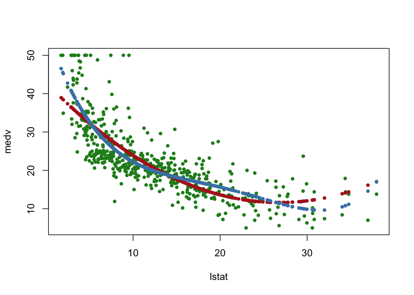
plot(medv ~ lstat, pch = 20, col = "forestgreen")
points(lstat, fitted(fit6), col = "firebrick", pch = 20)
fit7 = lm(medv ~ poly(lstat, 4), data = Boston)
points(lstat, fitted(fit7), col = "steelblue", pch = 20)

9 Qualitative Predictors and Interaction Terms

For qualitative predictors, we use the Carseats dataset and explore how different factors affect sales.

## Qualitative Predictors and Interaction Terms

# Load the Carseats dataset
data(Carseats)
attach(Carseats)

# Proceed with the rest of the analysis
names(Carseats)
 [1] "Sales"       "CompPrice"   "Income"      "Advertising" "Population" 
 [6] "Price"       "ShelveLoc"   "Age"         "Education"   "Urban"      
[11] "US"         
summary(Carseats)
     Sales          CompPrice       Income        Advertising    
 Min.   : 0.000   Min.   : 77   Min.   : 21.00   Min.   : 0.000  
 1st Qu.: 5.390   1st Qu.:115   1st Qu.: 42.75   1st Qu.: 0.000  
 Median : 7.490   Median :125   Median : 69.00   Median : 5.000  
 Mean   : 7.496   Mean   :125   Mean   : 68.66   Mean   : 6.635  
 3rd Qu.: 9.320   3rd Qu.:135   3rd Qu.: 91.00   3rd Qu.:12.000  
 Max.   :16.270   Max.   :175   Max.   :120.00   Max.   :29.000  
   Population        Price        ShelveLoc        Age          Education   
 Min.   : 10.0   Min.   : 24.0   Bad   : 96   Min.   :25.00   Min.   :10.0  
 1st Qu.:139.0   1st Qu.:100.0   Good  : 85   1st Qu.:39.75   1st Qu.:12.0  
 Median :272.0   Median :117.0   Medium:219   Median :54.50   Median :14.0  
 Mean   :264.8   Mean   :115.8                Mean   :53.32   Mean   :13.9  
 3rd Qu.:398.5   3rd Qu.:131.0                3rd Qu.:66.00   3rd Qu.:16.0  
 Max.   :509.0   Max.   :191.0                Max.   :80.00   Max.   :18.0  
 Urban       US     
 No :118   No :142  
 Yes:282   Yes:258  


fit1 = lm(Sales ~ . + Income:Advertising + Age:Price, data = Carseats)
summary(fit1)

Call:
lm(formula = Sales ~ . + Income:Advertising + Age:Price, data = Carseats)

Residuals:
    Min      1Q  Median      3Q     Max 
-2.9208 -0.7503  0.0177  0.6754  3.3413 

Coefficients:
                     Estimate Std. Error t value Pr(>|t|)    
(Intercept)         6.5755654  1.0087470   6.519 2.22e-10 ***
CompPrice           0.0929371  0.0041183  22.567  < 2e-16 ***
Income              0.0108940  0.0026044   4.183 3.57e-05 ***
Advertising         0.0702462  0.0226091   3.107 0.002030 ** 
Population          0.0001592  0.0003679   0.433 0.665330    
Price              -0.1008064  0.0074399 -13.549  < 2e-16 ***
ShelveLocGood       4.8486762  0.1528378  31.724  < 2e-16 ***
ShelveLocMedium     1.9532620  0.1257682  15.531  < 2e-16 ***
Age                -0.0579466  0.0159506  -3.633 0.000318 ***
Education          -0.0208525  0.0196131  -1.063 0.288361    
UrbanYes            0.1401597  0.1124019   1.247 0.213171    
USYes              -0.1575571  0.1489234  -1.058 0.290729    
Income:Advertising  0.0007510  0.0002784   2.698 0.007290 ** 
Price:Age           0.0001068  0.0001333   0.801 0.423812    
---
Signif. codes:  0 '***' 0.001 '**' 0.01 '*' 0.05 '.' 0.1 ' ' 1

Residual standard error: 1.011 on 386 degrees of freedom
Multiple R-squared:  0.8761,    Adjusted R-squared:  0.8719 
F-statistic:   210 on 13 and 386 DF,  p-value: < 2.2e-16
contrasts(Carseats$ShelveLoc)
       Good Medium
Bad       0      0
Good      1      0
Medium    0      1

10 Custom Regression Plot Function

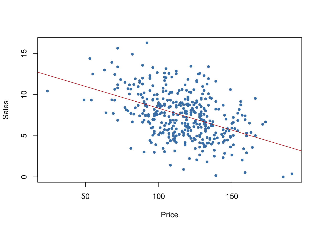
Finally, we create a custom function to simplify plotting regression models.

regplot = function(x, y, ...){
  fit = lm(y ~ x)
  plot(x, y, ...)
  abline(fit, col = "firebrick")
}

regplot(Price, Sales, xlab = "Price", ylab = "Sales", col = "steelblue", pch = 20)

11 Conclusion

In this lab, we have covered the basics of linear regression, including simple and multiple regression models, interaction terms, and nonlinear relationships. We also explored working with qualitative predictors and developed a custom plotting function for regression analysis.

Back to top