# install.packages(c("caret", "dplyr", "ggplot2", "tidyr"))
library(caret)
library(dplyr)
library(tidyr)
library(ggplot2)Lab08 caret Random Forest, KNN, GLMNet
1 Knowledge Mining: caret - Random Forest, KNN, GLMNet
In this lab, we will focus on the caret package and its use for building Random Forest models. Random Forest is an ensemble learning method that constructs multiple decision trees and averages their results to provide accurate and generalized predictions. While the code in this lab demonstrates Random Forest, similar approaches can be applied using other models like K-Nearest Neighbors (KNN) and GLMNet.
KNN is a simple, instance-based learning algorithm that works well for smaller datasets but can struggle with larger ones, whereas GLMNet applies regularization techniques to handle high-dimensional data effectively. These methods offer different advantages depending on the problem and dataset at hand.
We reference the works of Kuhn et al. (2008) and the caret documentation (2020) for additional insight into building predictive models.
1.1 Load Required Libraries
2 Example 1: Random Forest Classification with the Iris Dataset
We will use the iris dataset to demonstrate the implementation of a classification model using Random Forests.
2.1 Data Preparation
First, load the iris dataset and visualize the relationship between Sepal length, width, and species.
# Load the iris dataset
data(iris)

# Examine the dataset
head(iris)
Sepal.Length Sepal.Width Petal.Length Petal.Width Species
1 5.1 3.5 1.4 0.2 setosa
2 4.9 3.0 1.4 0.2 setosa
3 4.7 3.2 1.3 0.2 setosa
4 4.6 3.1 1.5 0.2 setosa
5 5.0 3.6 1.4 0.2 setosa
6 5.4 3.9 1.7 0.4 setosa# Data visualization
ggplot(iris, aes(x = Sepal.Length, y = Sepal.Width, color = Species)) +
geom_point() +
theme_bw()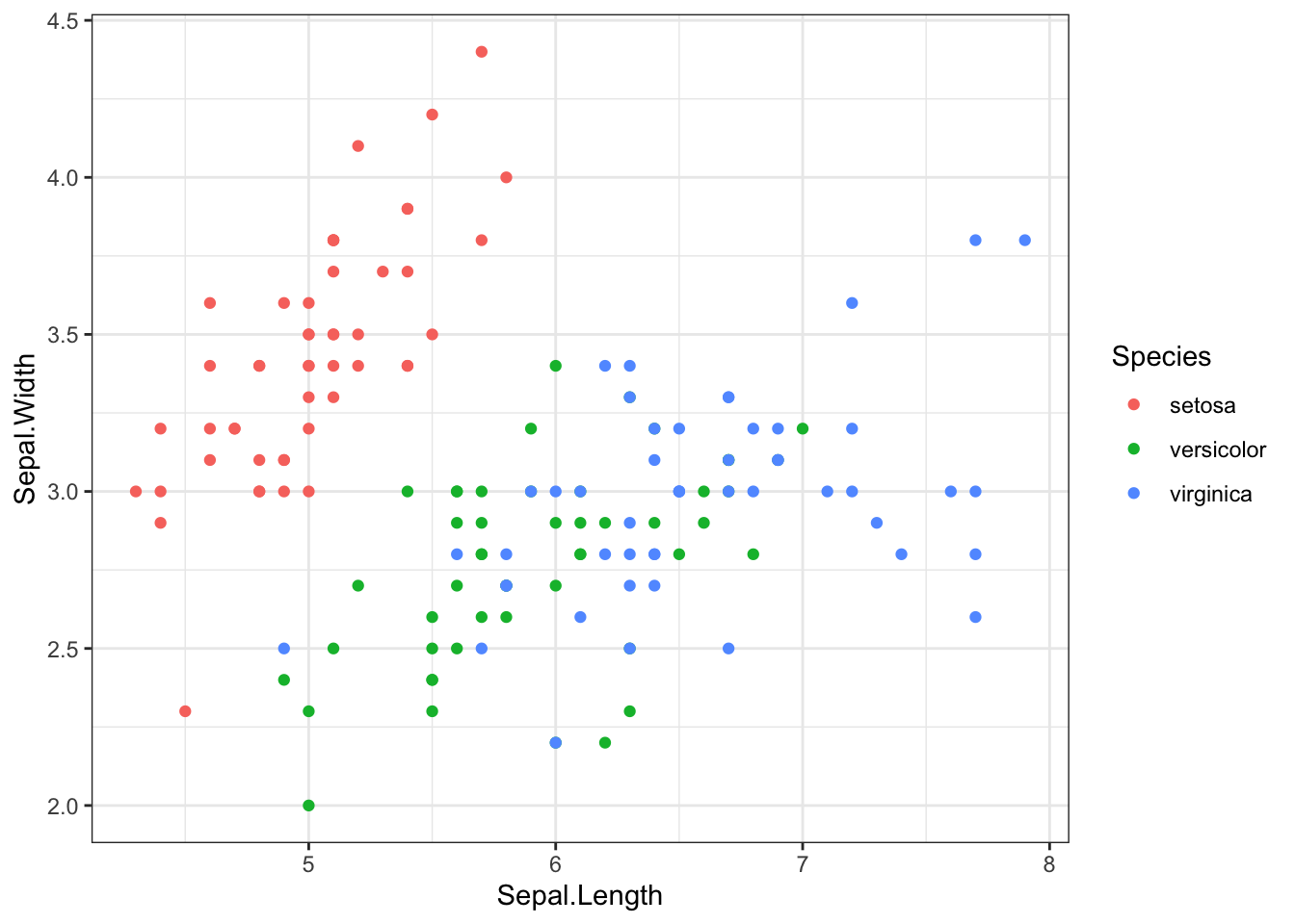
2.2 Train/Test Split
Next, split the data into a training set (70%) and a testing set (30%).
# Split the data into training and testing sets (70% train, 30% test)
set.seed(123)
train_index <- sample(1:nrow(iris), 0.7 * nrow(iris))
train_data <- iris[train_index, ]
test_data <- iris[-train_index, ]
2.3 Train the Random Forest Model
We set up 10-fold cross-validation and train the model using the train() function from the caret package.
# Set up the training control
train_control <- trainControl(method = "cv", number = 10) # 10-fold Cross-Validation

# Train the model
set.seed(123)
model <- caret::train(Species ~ ., data = train_data,
               method = "rf", # Random Forest
               trControl = train_control,
               tuneLength = 3,
               preProcess = c("center", "scale"))

# Print the model details
print(model)
Random Forest
105 samples
4 predictor
3 classes: 'setosa', 'versicolor', 'virginica'
Pre-processing: centered (4), scaled (4)
Resampling: Cross-Validated (10 fold)
Summary of sample sizes: 95, 95, 95, 95, 93, 95, ...
Resampling results across tuning parameters:
mtry Accuracy Kappa
2 0.9518182 0.9274934
3 0.9518182 0.9274934
4 0.9518182 0.9274934
Accuracy was used to select the optimal model using the largest value.
The final value used for the model was mtry = 2.2.4 Evaluate the Model
Finally, predict the species for the test data and calculate the accuracy of the model.
# Make predictions on the test data
predictions <- predict(model, test_data)

# Calculate the accuracy of the model
accuracy <- mean(predictions == test_data$Species)
cat("Accuracy:", accuracy)
Accuracy: 0.97777783 Example 2: Random Forest Regression with the mtcars Dataset
Now, we will demonstrate regression using the mtcars dataset.
3.1 Data Preparation
Load the dataset and split it similarly to the previous example.
# Load the mtcars dataset
data(mtcars)

# Examine the dataset
head(mtcars)
mpg cyl disp hp drat wt qsec vs am gear carb
Mazda RX4 21.0 6 160 110 3.90 2.620 16.46 0 1 4 4
Mazda RX4 Wag 21.0 6 160 110 3.90 2.875 17.02 0 1 4 4
Datsun 710 22.8 4 108 93 3.85 2.320 18.61 1 1 4 1
Hornet 4 Drive 21.4 6 258 110 3.08 3.215 19.44 1 0 3 1
Hornet Sportabout 18.7 8 360 175 3.15 3.440 17.02 0 0 3 2
Valiant 18.1 6 225 105 2.76 3.460 20.22 1 0 3 1# Split the data into training and testing sets (70% train, 30% test)
set.seed(123)
train_index <- sample(1:nrow(mtcars), 0.7 * nrow(mtcars))
train_data <- mtcars[train_index, ]
test_data <- mtcars[-train_index, ]3.2 Train the Random Forest Model
We now train a random forest regression model to predict the mpg variable.
# Set up the training control
train_control <- trainControl(method = "cv", number = 10)

# Train the regression model
set.seed(123)
model <- train(mpg ~ ., data = train_data,
               method = "rf",
               trControl = train_control,
               tuneLength = 3,
               preProcess = c("center", "scale"))

# Print the model details
print(model)
Random Forest
22 samples
10 predictors
Pre-processing: centered (10), scaled (10)
Resampling: Cross-Validated (10 fold)
Summary of sample sizes: 19, 20, 20, 20, 20, 20, ...
Resampling results across tuning parameters:
mtry RMSE Rsquared MAE
2 2.796874 0.9759378 2.437864
6 2.636784 0.9765995 2.276657
10 2.627549 0.9745273 2.270757
RMSE was used to select the optimal model using the smallest value.
The final value used for the model was mtry = 10.3.3 Evaluate the Model
Evaluate the model’s performance using the Root Mean Squared Error (RMSE) on the test data.
# Make predictions on the test data
predictions <- predict(model, test_data)

# Calculate the RMSE (Root Mean Squared Error) of the model
RMSE <- sqrt(mean((predictions - test_data$mpg)^2))
cat("RMSE:", RMSE)
RMSE: 2.0036344 Conclusion
In this lab, we demonstrated how to use the caret package to train and evaluate Random Forest models for both classification and regression tasks. By splitting the data, setting up cross-validation, and using caret’s train() function, we efficiently built models for both the iris and mtcars datasets. The results demonstrate the utility of Random Forests for predictive tasks.
While Random Forest is ideal for handling complex data and preventing overfitting, alternative methods like KNN and GLMNet offer their own benefits. KNN is intuitive and works well for small datasets, and GLMNet applies regularization to manage high-dimensional data. By understanding these models, we can choose the best approach based on the problem’s requirements and the dataset’s structure.
5 References
- Kuhn, Max. 2008. “Building predictive models in R using the caret package.” Journal of Statistical Software 28: 1-26.
- Kuhn, Max, et al. “Package ‘caret’.” The R Journal 223, no. 7 (2020).
- caret Documentation